Term Project: Land change in the Fraser Valley region of Abbotsford, British Columbia

Introduction
For my term project I chose to perform four different remote sensing techniques on landsat images of my hometown of Abbotsford, British Columbia. Which is located along the Fraser River in the province of British Columbia, Canada. This area is located in the river valley, which is commonly referred to as the Fraser Valley region and is a host to many cities and suburbs. The river valley runs from the Rocky Mountains to the Georgia Strait, and hosts British Columbia's capital city Vancouver. I chose to look at land use change in this area, by looking at three time periods: 2008, 2011 and 2013.

Methods
All images were obtained from the global viewer by the USGS or glovis. These images were imported into Erdas imagine and stacked with layer stacking to create ERDAS files. To begin my project, the first technique I chose to employ was image subset. To do this I used ArcGIS online to find a shapefile of the census regions in B.C., of which the Fraser Valley is one. I then selected Fraser Valley census region and exported its information to create a shapefile. The shapefile was quite large and covered more area than I wanted to show, so I used the editor toolbar in ArcMap and cut the shapefile in half. This shapefile was then used in Erdas Imagine to create an area of interest, which was used to create the image subset.

The next technique that I used was pan-sharpening. This technique uses a panchromatic band 8, which has a resolution of 15 m to increase the resolution of a regular multispectral landsat image, which originally has a resolution of 30 m. Erdas imagine has a specific tool to create a pansharpened output image. landsat 4 and 5 did not include a panchromatic band, so for this technique I used the recently instated landsat 8 satellite.

To see land change however I employed two specific techniques, the normalized difference vegetation index (NDVI) and binary change detection. NDVI find the areas with vegetation and makes them white or shades of grey. Using two images from different years, NDVI can be used to detect changes in vegetation. For example the next image shows a top of a hill that is favorable for subdivision expansion. In 2008, there is some expansion but the difference is visible in 2012 (view the white blotch in the middle, it has more dark areas in 2011 indicating loss of vegetation).

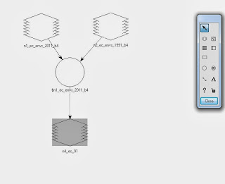
The final technique was binary change detection which subtracts the older year from the younger year and reclassifies the areas where change occured so it appears as white, and no change as black. This classification image was then input into ArcMap and the black made hollow and white made red, so that we can see the areas with significant change overlaid over a image of the city.

The final result is that the majority of change occured over the agricultural areas, as can be expected as farmers change out fields or let them grow fallow for the season.. Some areas near the city however are interesting and indicate urban growth, especially atop the hillls and within the city.

Lab 5 Image mosaic and Miscellaneous image functions 2

Goals and Objectives

The purpose of this lab is to introduce analytical processes in remote sensing. The objective of this lab is to explore techniques such as RGB to IHS transformation, image mosaicking, spatial and spectral enhancement, band ratio, and binary change detection.

Part 1 RGB to IHS and back
For this part of the lab we looked at a normal RGB image and transformed it to IHS, and then back again to RGB to improve the histograms.

Part 2 Image Mosaicking.

Part 5 Binary Change Detection

Figure 1 Binary change detection output image. This image was created after running the Raster tool Functions - Two Image functions. What this does is subtracts the brightness values of an older image from that of a newer image to obtain this result.

Figure 2 Model Maker to perform the same result as Figure 1

Lab 8 Spectral Signature Analysis

Introduction
For this lab we looked at the spectral signatures that objects produce, which aids in analysis. Each object reflects light in a different manner, some absorb certain wavelengths and refelect others, creating a unique signature that can be used to idenify objects. Using a landsat image of Eau Claire, we collected spectral signatures with the signature editor tool in Erdas Imagine. Tweleve signatures were collected: Standing water, moving water, vegetation, riparian vegetation, crops, urban grass, uncultivated moist soil, dry soil, rock, parking lot, asphalt highway, and airport runway.

 

Most plant signatures are moderate in the blue and green bands but then increases significantly in the red and near infrared bands, this allows them to absorb green light energy and reflect harmful red and near infrared light, which can cause cell damage. Water signatures are higher in the blue band but then decrease significantly in the near infrared band as it absorbs the infrared light. Rock surfaces tend to absorb red and near infrared light, but reflect blue green and red light.

 

Overall this was a very interesting lab because it shows how remote sensing analysis can be used for image classification and analysis.

Lab 7 - Introduction to Photogrammetry

Goals and Objectives
The purpose of this lab is to introduce the class to photogrammetry techniques and stereoscopy. Part one involves looking at scales and measurement as well as relief displacement, part two involves creating and looking at stereoscopic images, and part three involves orthorectification.

Part 1
For part one we looked at images of Eau Claire, WI in Erdas Imagine. Using the measurement tool and hand rulers, we measured actual images and calculated perimiter, as well as relief displacement. With displacement something like a smoke stack may appear at a more oblique view (side view), with relief displacement, we find the principle point of the image and measure to the object, calculating displacement and correcting.

Part 2
For this part we looked at stereoscopy. We created an anaglyph image of Eau Claire, which requires 3D glasses to view. Using this image we can visualize easier elevation and buildings. In order to create this image, we used a digital elevation model to produce ground control points.

Part 3
For this part of the lab we looked at orthorectification. Using Erdas Imagine Lecia Photogrammetric Suite (LPS), we created an accuate set of ground control points to rectify an image.